MS EXCEL - Freeze Pane
MS EXCEL - Freeze Pane
Used to keep an area of a worksheet visible while you scroll to another area of the worksheet, you can lock specific rows or columns in one area by freezing or splitting panes.
You may want to see certain rows or columns all the time in your worksheet, especially header cells.
By freezing rows or columns in place, you’ll be able to scroll through your content while continuing to view the frozen cells.
1. Select the row below the row(s) you want to freeze.
2. Click the View tab on the Ribbon.
3. Select the Freeze Panes command, then choose Freeze Panes from the drop-down menu.
The rows will be frozen in place, as indicated by the gray line. You can scroll down the worksheet while continuing to view the frozen rows at the top. Repeat the same for column freezing.
To unfreeze rows or columns, click the Freeze Panes command, then select Unfreeze Panes from the drop-down menu.
MS EXCEL - Formatting in Excel
MS EXCEL - Formatting in Excel
Formatting is available under Home Tab in Excel
Format Painter - Used to Copy formatting from one Cell/Range to other. Double click this
option to apply multiple time
Font Formatting - It consists of Font Name, Size and Bold/Italics/Underline option
Border Formatting - It allows you to modify cell borders
Text Formatting - It has various alignment option and Wrap Text option
Number Formatting - It gives various options of formatting Number like Currency,
Percentage, Decimals etc.
Table Formatting - Format table data, various styles available to choose from.
Cell Formatting (Cell Styles) - It allows to adjust height, width, insert and delete options
You can do formatting manually, by selecting fonts, font color and size, background colors and borders, or you can do the formatting quickly and automatically using styles. A style is a mixture of formatting that you can apply over and over, like paint.
MS EXCEL - Sheet Protection, Share workbook, Workbook Protection
MS EXCEL - Sheet Protection, Share workbook, Workbook Protection
I. Worksheet Level Protection and Locking/Unlocking of Cell
1. SELECT THE CELL AND THEN RIGHT CLICK
2. CHOOSE Format Cells -> Protection

NOTE: Make sure to lock the cells before you protect the sheet or document. Once a sheet or a document has been protected, you cannot access menu selections that allow you to make changes to cells.
In Menu bar go to Review - Protect Sheet -> Give Password and select/unselect the various access for user

II. Workbook Level Protection
You can prevent a workbook from having its structure and windows modified or resized by another user.
Structure
Prevents the user from changing the order of the sheets within a workbook. This includes adding or deleting worksheets.
Windows
Prevents the user from being able to resize or move the window.

III. File Level Protection
To password protect Excel file - Save as - Tools - General Options and can give password here to open and edit.


OPTIONAL: If you would like Excel to recommend that this file be opened as a read-only file each time it is opened, select Read-only recommended

HINT: Read-only files can be modified, but the changes cannot be saved without creating a new file.
If you no longer need to password-protect the file, you can remove the password by going to save As -> Tools -> and delete the current password, save it and replace old file.
MS EXCEL - Text to Column
Text to Column
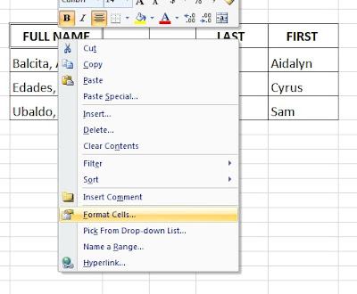
To separate the contents of one Excel cell into separate columns, you can use the ‘Convert
Text to Columns Wizard’.
For example - when you want to separate a list of full names into last and first
names.

1. Select the range with full names.
2. On the Data tab, click Text to Columns.
The following dialog box appears.

3. Choose Delimited and click Next.
4. Clear all the check boxes under Delimiters except for the Comma and Space check box.
5. Click Finish.
MS EXCEL - Validation
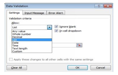
Data Validation - It allows you to define validation on cells for entering value.
Common Validations are - List, Date, Time, Text Length etc.
List Validation - It will create a drop down containing a range or defined values
Select the Cell/Range to Validate -> Goto Data -> Data Validation -> select the Validation criteria here and press OK. Now cell will take only defined values
Circle Invalid Data - It will put circle on cell containing Invalid values, when validation is defined after entering values.
Subscribe to:
Posts (Atom)