MS EXCEL - Freeze Pane
MS EXCEL - Freeze Pane
Used to keep an area of a worksheet visible while you scroll to another area of the worksheet, you can lock specific rows or columns in one area by freezing or splitting panes.
You may want to see certain rows or columns all the time in your worksheet, especially header cells.
By freezing rows or columns in place, you’ll be able to scroll through your content while continuing to view the frozen cells.
1. Select the row below the row(s) you want to freeze.
2. Click the View tab on the Ribbon.
3. Select the Freeze Panes command, then choose Freeze Panes from the drop-down menu.
The rows will be frozen in place, as indicated by the gray line. You can scroll down the worksheet while continuing to view the frozen rows at the top. Repeat the same for column freezing.
To unfreeze rows or columns, click the Freeze Panes command, then select Unfreeze Panes from the drop-down menu.
MS EXCEL - Formatting in Excel
MS EXCEL - Formatting in Excel
Formatting is available under Home Tab in Excel
Format Painter - Used to Copy formatting from one Cell/Range to other. Double click this
option to apply multiple time
Font Formatting - It consists of Font Name, Size and Bold/Italics/Underline option
Border Formatting - It allows you to modify cell borders
Text Formatting - It has various alignment option and Wrap Text option
Number Formatting - It gives various options of formatting Number like Currency,
Percentage, Decimals etc.
Table Formatting - Format table data, various styles available to choose from.
Cell Formatting (Cell Styles) - It allows to adjust height, width, insert and delete options
You can do formatting manually, by selecting fonts, font color and size, background colors and borders, or you can do the formatting quickly and automatically using styles. A style is a mixture of formatting that you can apply over and over, like paint.
MS EXCEL - Sheet Protection, Share workbook, Workbook Protection
MS EXCEL - Sheet Protection, Share workbook, Workbook Protection
I. Worksheet Level Protection and Locking/Unlocking of Cell
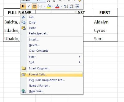
1. SELECT THE CELL AND THEN RIGHT CLICK

2. CHOOSE Format Cells -> Protection
NOTE: Make sure to lock the cells before you protect the sheet or document. Once a sheet or a document has been protected, you cannot access menu selections that allow you to make changes to cells.
In Menu bar go to Review - Protect Sheet -> Give Password and select/unselect the various access for user
II. Workbook Level Protection
You can prevent a workbook from having its structure and windows modified or resized by another user.
Structure
Prevents the user from changing the order of the sheets within a workbook. This includes adding or deleting worksheets.
Windows
Prevents the user from being able to resize or move the window.
III. File Level Protection
To password protect Excel file - Save as - Tools - General Options and can give password here to open and edit.
OPTIONAL: If you would like Excel to recommend that this file be opened as a read-only file each time it is opened, select Read-only recommended
HINT: Read-only files can be modified, but the changes cannot be saved without creating a new file.
If you no longer need to password-protect the file, you can remove the password by going to save As -> Tools -> and delete the current password, save it and replace old file.
I. Worksheet Level Protection and Locking/Unlocking of Cell
1. SELECT THE CELL AND THEN RIGHT CLICK

2. CHOOSE Format Cells -> Protection
NOTE: Make sure to lock the cells before you protect the sheet or document. Once a sheet or a document has been protected, you cannot access menu selections that allow you to make changes to cells.
In Menu bar go to Review - Protect Sheet -> Give Password and select/unselect the various access for user
II. Workbook Level Protection
You can prevent a workbook from having its structure and windows modified or resized by another user.
Structure
Prevents the user from changing the order of the sheets within a workbook. This includes adding or deleting worksheets.
Windows
Prevents the user from being able to resize or move the window.
III. File Level Protection
To password protect Excel file - Save as - Tools - General Options and can give password here to open and edit.
OPTIONAL: If you would like Excel to recommend that this file be opened as a read-only file each time it is opened, select Read-only recommended
HINT: Read-only files can be modified, but the changes cannot be saved without creating a new file.
If you no longer need to password-protect the file, you can remove the password by going to save As -> Tools -> and delete the current password, save it and replace old file.
MS EXCEL - Text to Column
Text to Column
To separate the contents of one Excel cell into separate columns, you can use the ‘Convert
Text to Columns Wizard’.
For example - when you want to separate a list of full names into last and first
names.
1. Select the range with full names.
2. On the Data tab, click Text to Columns.
The following dialog box appears.
3. Choose Delimited and click Next.
4. Clear all the check boxes under Delimiters except for the Comma and Space check box.
5. Click Finish.
MS EXCEL - Validation
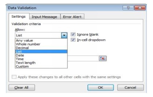
Data Validation - It allows you to define validation on cells for entering value.
Common Validations are - List, Date, Time, Text Length etc.
List Validation - It will create a drop down containing a range or defined values
Select the Cell/Range to Validate -> Goto Data -> Data Validation -> select the Validation criteria here and press OK. Now cell will take only defined values

Circle Invalid Data - It will put circle on cell containing Invalid values, when validation is defined after entering values.
Common Validations are - List, Date, Time, Text Length etc.
List Validation - It will create a drop down containing a range or defined values
Select the Cell/Range to Validate -> Goto Data -> Data Validation -> select the Validation criteria here and press OK. Now cell will take only defined values

Circle Invalid Data - It will put circle on cell containing Invalid values, when validation is defined after entering values.
Chapter 2 - MS Excel
Chapter 2 - MS Excel
1. Important Date Functions (TODAY, NOW, YEAR, MONTH, DAY, DATE )
2. Age Calculations
3. Calculate End of Probation period using EDATE & WORKDAY
4. Calculate no. of working days between two dates (Networkdays Function)
5. Common Error types in Excel and error handling by Iferror function.
6. Substitute and Find
7. Left, Right and Mid
8. Common IS Functions : Istext, Isnumber, Isblank, Iserror
9. Len and Text
MS EXCEL - Common IS Functions : Istext, Isnumber, Isblank, Iserror
IS functions, checks the specified value and returns TRUE or FALSE depending on the
outcome.
EXAMPLE - isblank
MS EXCEL - Substitute and Find
MS EXCEL - Substitute and Find
=substitute(text,old, new)
Substitute old text with new text
EXAMPLE: Singh is replaced with kumari
“=SUBSTITUTE(A89,““Singh””,““Kumari””)“ Arti Kumari Chauhan
=Find(find_text,text) Find the position of one text within other text
EXAMPLE: g is at 9 position in Arti Singh Chauhan
9 =FIND(“g”,A89)
=substitute(text,old, new)
Substitute old text with new text
EXAMPLE: Singh is replaced with kumari
“=SUBSTITUTE(A89,““Singh””,““Kumari””)“ Arti Kumari Chauhan
=Find(find_text,text) Find the position of one text within other text
EXAMPLE: g is at 9 position in Arti Singh Chauhan
9 =FIND(“g”,A89)
MS EXCEL - Common Error types in Excel and error handling by Iferror function.
MS EXCEL - Common Error types in Excel and error handling by Iferror function.
#NAME? error
The #NAME? error occurs when Excel does not recognize text in a formula.
EXAMPLE: SU to SUM
#VALUE! error
Excel displays the #VALUE! error when a formula has the wrong type of argument.
#DIV/0! error
Excel displays the #DIV/0! error when a formula tries to divide a number by 0 or an empty cell.
#REF! error
Excel displays the #REF! error when a formula refers to a cell that is not valid.
EXAMPLE: Delete B column it will give error
MS EXCEL - Calculate no. of working days between two dates (Networkdays Function)
MS EXCEL - Calculate no. of working days between two dates (Networkdays Function)
Calculate employee benefits that accrue based on the number of days worked during a
specific term. The calculation includes all weekdays (Mon - Fri)
=NETWORKDAYS(startDate,endDate,[holidays])
holidays - [optional] A list of one or more dates that should be considered non-work days.
E.g- 25 Sept 2015 is written as 25
Note that the start_date, end_date and [holidays] arguments should be input as
either:
References to cells containing dates or Dates returned from formulas.
- If you attempt to input these date arguments as text, Excel may misinterpret them, due to
different date systems, or date interpretation settings Dates should be entered by using the DATE function, or as results of other formulas or functions. For example, use DATE(2012,5,23) for the 23rd day of May, 2012. Problems can occur if dates are entered as text.
MS EXCEL - Calculate End of Probation period using EDATE & WORKDAY
MS EXCEL - Calculate End of Probation period using EDATE & WORKDAY
Returns no of month before or after the start date.
=EDATE(Start_date,Months) , Months can be positive or negative.
So type in “=EDATE(“, click on the cell that contains their start date, type a comma, then
enter the number of months. 3 months? 6 months? Type a 3 or a 6 or whatever it is. Then
close your brackets “)” and press enter.
Done.
MS EXCEL - Age Calculations
MS EXCEL - Age Calculations
=datedif(d1,d2,“x”)
(input in cells)
D1- old date
D2- new date
x- It can be Y, M, D, YM, MD
Y- Return no of year between 2 dates
M- Return no. of months between 2 dates
D - Return no. of days between 2 dates
YM- Return no. of month in current year
MD- Return no of days in current months
Example –
Date1 - 10/29/1992 (Written in cell C14)
Date2 - 10/25/2015 (Written in cell C16)
=CONCATENATE(DATEDIF(C14,C16,“Y”),” Years “,DATEDIF(C14,C16,“YM”),”
Months “,DATEDIF(C14,C16,“MD”),” Days”)
22 Years 11 Months 26 Days
Important Date Functions (TODAY, NOW, YEAR, MONTH, DAY, DATE )
1. Important Date Functions (TODAY, NOW, YEAR, MONTH, DAY, DATE )
|
A
|
B
|
C
|
D
|
|
TODAY
|
Returns Current Date
|
=TODAY()
|
11/8/015
|
|
NOW
|
Returns Current Date
|
=NOW()
|
11/29/2015
17:43
|
|
MONTH
|
Returns numeric month from date
|
=MONTH (D4)
|
11
|
|
YEAR
|
Returns year in YYYY format
from date
|
=YEAR(D4)
|
2015
|
|
DAY
|
Returns numeric day from date
|
=DAY(D4)
|
29
|
|
DATE
|
=DATE(YEAR,MONTH,DAY)
|
=DATE(2015,4,1)
|
4/1/2015
|
Count Functions in MS Excel
Count Functions in MS Excel
Count, Counta, Countblank, Countif
Count - Count only numeric value in a range not text
Counta- Calculates all except blank and including space in a range
Countif - Count no. of cell within a range that meet the given condition.
Countblank - Count blank cells space will be counted as zero.
Count, Counta, Countblank, Countif
Count - Count only numeric value in a range not text
Counta- Calculates all except blank and including space in a range
Countif - Count no. of cell within a range that meet the given condition.
Countblank - Count blank cells space will be counted as zero.
Concatenate in MS Excel
Concatenate in MS Excel
CONCATENATE is a text function used to join two or more text strings into one string.
Syntax: CONCATENATE(text1, [text2], …)
CONCATENATE is a text function used to join two or more text strings into one string.
Syntax: CONCATENATE(text1, [text2], …)
Format Painter in MS Excel
Format Painter in MS Excel
Format Painter copies formatting from one place and applies it to another quickly. It is usefull in Tables, Value and Header formatting. Double click the Format Painter button to apply the same formatting to multiple cells.
FIRST 10 MS EXCEL KEYBOARD SHORTCUTS
FIRST 10 EXCEL MS KEYBOARD SHORTCUTS
1. Ctrl+Z Undo
2. Ctrl+Y Redo
3. Ctrl+C Copy
4. Ctrl+V Paste
5. Ctrl+S Save
6. Ctrl+N New Workbook
7. Ctrl+O Open
8. Ctrl+F Find
9. Ctrl+P Print
10. Ctrl+A Select All
1. Ctrl+Z Undo
2. Ctrl+Y Redo
3. Ctrl+C Copy
4. Ctrl+V Paste
5. Ctrl+S Save
6. Ctrl+N New Workbook
7. Ctrl+O Open
8. Ctrl+F Find
9. Ctrl+P Print
10. Ctrl+A Select All
SUM, AVERAGE, PRODUCT, POWER (AN INTRODUCTION TO EXCEL MATH FUNCTIONS)
MS Excel Math Functions
SUM, AVERAGE, PRODUCT, POWER
SUM, AVERAGE, PRODUCT, POWER
Formula
|
Input
|
Output
|
SUM
|
=SUM(3,4,5)
|
12
|
AVERAGE
|
=AVERAGE(2,4,6)
|
4
|
PRODUCT
|
=PRODUCT(2,3,4)
|
24
|
CARET
|
=POWER(2,2)
|
4
|
MS EXCEL- Relative Reference and Absolute Reference
MS EXCEL- Relative Reference and Absolute Reference
Relative references
A relative cell reference in a formula, such as A1, is based on the relative position of the cell that contains the formula and the cell the reference refers to. If the position of the cell that contains the formula changes, the reference is changed. If you copy or fill the formula across rows or down columns, the reference automatically adjusts. By default, new formulas use relative references.
For example, if you copy or fill a relative reference in cell D5 to cell D6, it automatically adjusts from =B5*C5 (shown in the above photo) to =B6*C6 (shown below.)
Absolute references
An absolute cell reference in a formula, such as $E$4, always refer to a cell in a specific location. If the position of the cell that contains the formula changes, the absolute reference remains the same. If you copy or fill the formula across rows or down columns, the absolute reference does not adjust. By default, new formulas use relative references, so you may need to switch them to absolute references. For example, if you copy or fill an absolute reference in cell D6 to cell D7, it stays the same in both cells: =$E$4.
For example, if you copy or fill an absolute reference in cell D6 to cell D7, the relative cells automatically adjusts from =(B6*C6)*$E$4 to =(B6*C6)*$E$4, however notice that the absolute reference remains the same in both cells: =$E$4.
Operators in MS Excel
Operators in MS Excel
There are four different types of Operators in Excel: Arithmetic, Comparison, Text Concatenation and Reference.
Arithmetic Operators
To perform basic mathematical operations, such as addition, subtraction, multiplication, or division; combine numbers; and produce numeric results,use the following arithmetic operators.
Arithmetic
Operator
|
Meaning
|
Operation
Performed
|
Output
|
+ (plus sign)
|
Addition
|
3+3
|
6
|
- (minus sign)
|
Subtraction
|
3-1
|
2
|
-
|
Negation
|
-1
|
-1
|
* (asterisk)
|
Multiplication
|
3*3
|
9
|
/ (forward slash)
|
Divison
|
3/2
|
1.5
|
% (percent sign)
|
Percent
|
20%
|
.20
|
^ (caret)
|
Exponentiation
|
3^2
|
9
|
Comparison Operators
You can compare two values with the following operators. When two values are compared by using these operators, the result is a logical value -either TRUE or FALSE.
Comparison
Operator
|
Meaning
|
Example
|
= (equal sign)
|
Equal
to
|
A1=B1
|
> (greater than sign)
|
Greater
than
|
A1>B1
|
< (less than sign)
|
Less
than
|
A1<B1
|
>= (greater than or equal to sign)
|
Greater
than or Equal to
|
A1>=B1
|
<= (greater than or equal to sign)
|
Less
than or Equal to
|
A1<=B1
|
<> (not equal to sign)
|
Not
Equal to
|
A1<>B1
|
Text Concatenation Operator
Use the ampersand (&) to concatenate (join) one or more text strings to produce a single piece of text.
Text
Operator
|
Meaning
|
Example
|
& (ampersand)
|
Connects,
or concatenates, two values to produce one continuous text value
|
"North" & "Wind"
results in "Northwind"
|
Reference Operators in MS Excel
Combine ranges of cells for calculations with the following operators.
Note: AND,OR etc are logical functions not logical operators as they return value on passing arguments.
BACK TO CHAPTER 1
Combine ranges of cells for calculations with the following operators.
Reference Operator
|
Meaning
|
Example
|
: (colon)
|
Range operator, which produces one
reference to all the cells between two
references, including the two
references.
|
B5:B15
|
, (comma)
|
Union operator, which combines
multiple references into one reference
|
SUM(B5:B15,D5:D15)
|
(space)
|
Intersection operator, which produces
one reference to cells common to the
two references
|
B7:D7 C6:C8
|
Note: AND,OR etc are logical functions not logical operators as they return value on passing arguments.
BACK TO CHAPTER 1
Subscribe to:
Comments (Atom)


